def initial_clean(text):
    text = re.sub(r'[^\w\s]','',text)
    text = text.lower() 
    text = nltk.word_tokenize(text)
    return text
 
stop_words = stopwords.words('english')
def remove_stop_words(text):
    return [word for word in text if word not in stop_words]
 
stemmer = PorterStemmer()
def stem_words(text):
    try:
        text = [stemmer.stem(word) for word in text]
        text = [word for word in text if len(word) > 1] 
    except IndexError: 
        pass
    return text
 
def apply_all(text):
    return stem_words(remove_stop_words(initial_clean(text)))

df['clean_text'] = df['text'].apply(apply_all) 
df

Here, it is straightforward to see the difference between the text before and after the preprocessing operations.

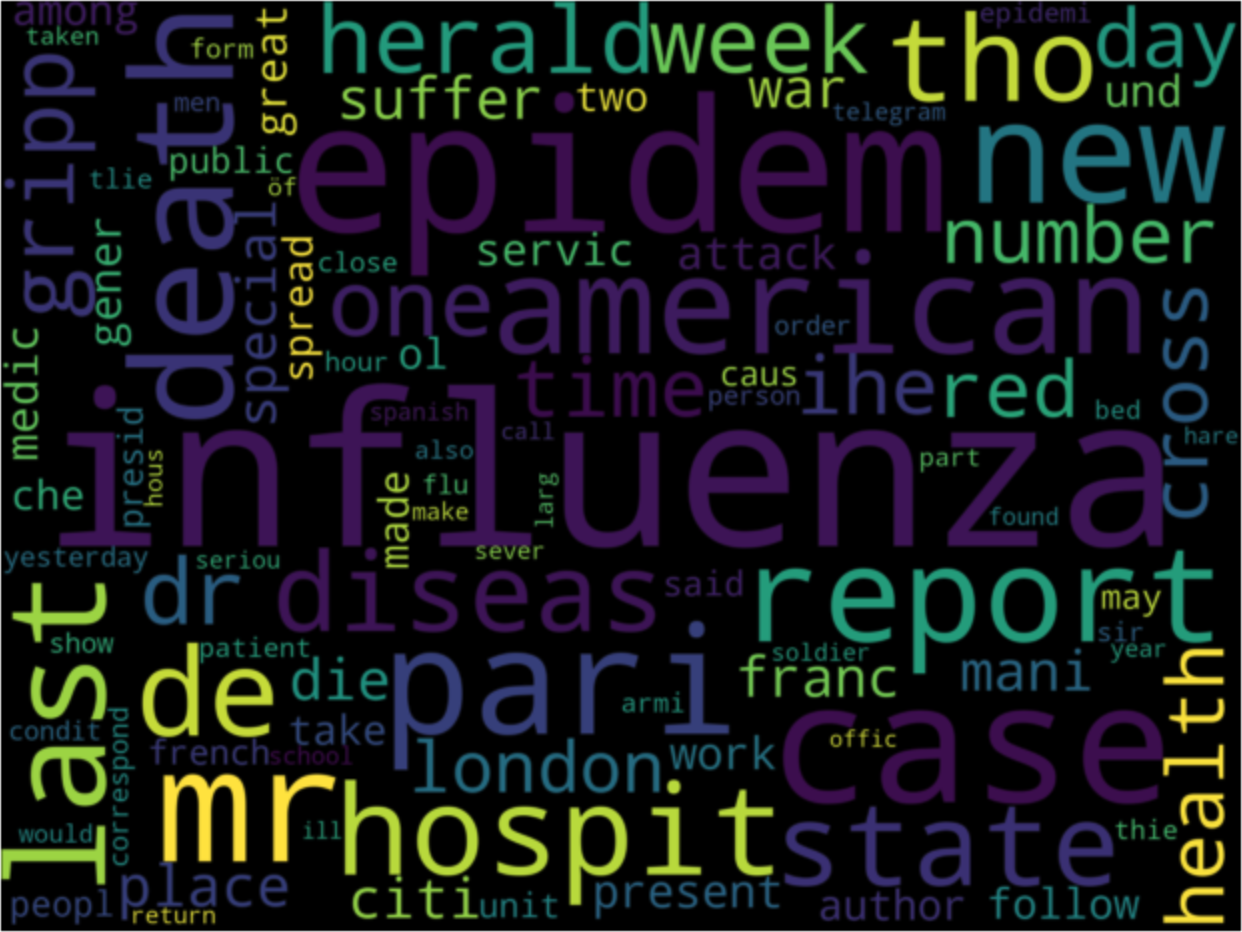
But what can we do to understand what our corpus contains? One way to graphically represent a corpus is to create a word cloud.

A word cloud is a visual representation of text data in which the size of each word indicates its frequency or importance in the text. Words that appear more frequently in the text are displayed with a larger font size, while less frequent words are smaller. Word clouds are useful for quickly identifying the most common themes or topics in a text corpus.

This representation can help gain a high-level understanding of the main topics or themes present in the corpus. Analyzing the word cloud makes it possible to identify which words or phrases are most frequently mentioned in the text and which are less common. This can provide insights into the main subjects covered in the corpus and help to guide further analysis.

To build this word cloud, we are using N-grams. N-grams are useful in humanities discourse analysis because they can reveal patterns of language use and help identify the most common words and phrases used in a given corpus. This can provide insight into the topics being discussed; the language style used, and even the social and cultural context in which the language was produced.

For example, in literary studies, analyzing the frequency and context of certain words or phrases can reveal patterns of character development or plot structure. In political discourse analysis, N-grams can be used to analyze the language used by political leaders and identify patterns of rhetoric or manipulation.

Here is the code to display a word cloud. Feel free to analyze each line of the code : 

# Create a list of bigrams from the clean_text column in the dataframe
bigrams_list = list(nltk.bigrams(df['clean_text']))
 
# Create a dictionary containing the bigrams as a single string
dictionary = [' '.join([str(tup) for tup in bigrams_list])]
 
# Use CountVectorizer to create a bag of words from the dictionary
vectorizer = CountVectorizer(ngram_range=(1, 1))
bag_of_words = vectorizer.fit_transform(dictionary)
 
# Get the vocabulary from the vectorizer
vectorizer.vocabulary_
 
# Sum the words in the bag of words
sum_words = bag_of_words.sum(axis=0)
 
# Create a list of tuples containing the word and its frequency
words_freq = [(word, sum_words[0, idx]) for word, idx in vectorizer.vocabulary_.items()]
 
# Sort the list by frequency in descending order
words_freq =sorted(words_freq, key = lambda x: x[1], reverse=True)
 
# Convert the list of tuples to a dictionary
words_dict = dict(words_freq)
 
# Set parameters for the wordcloud
WC_height = 1500
WC_width = 2000
WC_max_words = 100
 
# Create the wordcloud using WordCloud library and generate it from the dictionary of words
wordCloud = WordCloud(max_words=WC_max_words, height=WC_height, width=WC_width)
wordCloud.generate_from_frequencies(words_dict)
 
# Plot the wordcloud
plt.figure(figsize=(8,8))
plt.plot
plt.imshow(wordCloud, interpolation='bilinear')
plt.axis("off")
plt.show()